Investing After a Liquidity Event

August 16, 2026 —

The recent IPO of SpaceX and the anticipated IPOs of Anthropic and OpenAI are focusing attention on how to invest following a liquidity event. We discuss several important decision points.

Introduction

Those who recently experienced a liquidity event have to make several important decisions:

What’s an appropriate risk target?
How do you construct a portfolio consistent with the risk target?
What role do alternative assets play in your portfolio?
What is a reasonable exercise strategy for existing option grants?

The rest of this piece focuses on these issues. There are, of course, other important things to consider, like designing an estate plan, potentially creating trusts, contributing to tax-advantaged accounts, and so on. We leave that discussion for another day.

Risk Tolerance

Investing in stocks and bonds involves risks, and regardless of how smart or experienced your advisor happens to be, these risks cannot be eliminated. Higher historical returns have been associated with higher historical risks. Taking risks intelligently should engender getting compensated for those risks on average, over time. This is how markets work. Rather than asking the question of what return you are trying to achieve, we advise clients to think about it from the other direction: What amount of risk are you comfortable holding in your portfolio? In particular, how much mark-to-market loss are you willing to bear in a market downturn? And for how long are you willing to see your portfolio well beneath its prior peak?

The risk question is complex because there are multiple risks to worry about. There are local risk measures which determine how much your portfolio is likely to fluctuate on a day-to-day basis. There are global risk measures which try to approximate how much your portfolio might lose in a very adverse market scenario. There is also liquidity risk, which determines how quickly and at what price you are able to turn parts or all of your investment portfolio to cash. A thorough analysis of this topic requires a discussion between you and your financial advisor about all of these different dimensions of risk and your willingness/ability to take them on.

Here we focus on only one aspect of risk, which is the historical drawdown of a portfolio. A drawdown is the peak-to-trough loss experienced by an investment portfolio. For example, if your portfolio reaches a value of $100 and then falls to $70, before turning around, that would be a drawdown of 30%. Using monthly data from January 1990 to July 2026, the next chart shows the pronounced relationship between historical returns (on the x-axis) and the historically worst drawdown of each portfolio (on the y-axis) during this time period. Each point on the graph represents the stock/bond mix of the portfolio. For example, 70/30 means a portfolio with 70% S&P 500 and 30% US medium-duration Treasuries, while 90/10 is 90% S&P 500 and 10% US Treasuries.

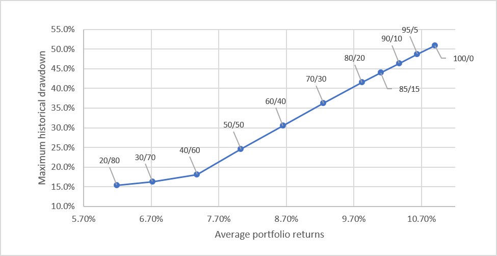
As the chart makes clear, the more stock-heavy portfolios have earned much higher returns historically, though at the cost of much higher historical drawdowns. The 70/30 portfolio earned a historical return in the January 1990 to July 2026 time period of 9.25%, with a worst-case historical drawdown of 36.2%. The riskier 90/10 portfolio earned a historical return of 10.37% with a worst-case historical drawdown of 46.4%.

There is another risk dimension which should be considered. This is the length of the drawdown, i.e., how long it took historically for a portfolio to set a new peak, following a drawdown from a prior peak. In our data, the longest drawdowns (those associated with the highest risk portfolios) lasted over 6 years, while the shortest drawdown (associated with the 30/70 portfolio) lasted 2.5 years. The next chart demonstrates this pattern.

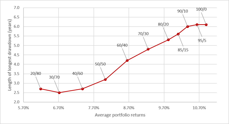
In discussing your portfolio allocation with your advisor, you should first settle on an appropriate risk level. If you want to minimize the chance that your $1,000,000 portfolio ever loses $500,000 in value, you should stay away from the 95/5 and 100/0 portfolios. If the most you can ever imagine losing is roughly 30% of your portfolio value, that puts you more in the 60/40 camp.

Keep in mind that both of these charts, which show the percent and length of drawdowns, present only historical numbers. Future returns across all risk levels may be considerably lower than these historical average returns. And future drawdowns may be much more severe, i.e., larger percent losses and longer-lasting. Also, using monthly data, as we do here, understates the drawdown the portfolio may experience on a day-to-day basis. So a 60/40 portfolio in the future may suffer a more severe drawdown than its historical, post-1990 worst-case level of 30.5%. Nevertheless the above figures are a useful guide for thinking about an appropriate risk level for your asset allocation plan.

Portfolio Implementation

Once you decide on an appropriate risk level for your portfolio, you need to think about how that portfolio should be implemented. At QuantStreet, we use a proprietary, systematic asset allocation approach. Our portfolios use low-cost, highly-liquid ETFs. We offer portfolios at many different risk levels, and also can customize portfolios to clients’ specific needs.

The next flowchart details our process. We begin with a machine-learning forecasting model for each of the 50 asset classes we track. The model customizes a forecasting model for each asset class based on a large number of potential forecasting variables (which include macroeconomic series, valuation and fundamental asset-class measures, among others). We combine the forecast of this model with the trend of each asset class, and feed this joint signal into our portfolio optimizer.

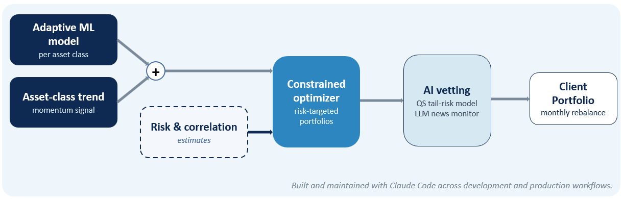
The optimizer takes information about volatility, correlation, and tail risks from historical estimates and combines these to answer the following question: At a given risk level, measured by both volatility and tail risk, what is the highest expected return portfolio that can be constructed given our risk and correlation estimates and the hybrid expected return signal coming from our machine learning model and the asset class trend? The portfolio optimizer also has many constraints that attempt to prevent oversized positions in a given asset class and enforce a certain amount of diversification.

Keep in mind that expected returns as used above is a term with a very specific, technical meaning. It is the mean return estimate produced by our forecasting model. The expected return is just an estimate, which is based on the information that we feed into our forecasting model. We have no idea what the future realized returns will actually look like across any of our asset classes. And future realized returns may deviate greatly, and negatively, from our expected return forecasts. Nevertheless, any portfolio optimizer needs its own set of capital market assumptions, and this is how we produce ours.

The proposed portfolios at each risk level then go through two rounds of AI-based vetting. One is a search through the last month’s newsflow (which we collect on a daily basis) to make sure that our proposed portfolios are not adversely affected by information that was outside of our machine learning forecasting process. This step is implemented using Gemini 3.5 Flash, accessed through our Google Cloud infrastructure. The second step asks our coding agent, which orchestrates many steps of our month-end rebalancing process, to do its own vetting of the proposed portfolio, taking the Gemini-generated news summary into consideration. This step is currently done by Claude Opus 5. We will update both models as new releases arrive. (Another example of how we use AI to monitor investment risks is our systemic risk dashboard, which we discussed in a Substack piece a few weeks back.)

The final step of the monthly rebalancing process is to enter the resultant portfolios from the above workflow into our portfolio rebalancing system (we use Schwab’s iRebal) and then rebalance each client’s account into the new risk-targeted monthly portfolio. There are many customizations that happen here for specific clients based on their particular circumstances.

Additional Considerations

There are several other portfolio considerations, which we now discuss.

Reduced Tech Exposure

Those working in the tech sector with stock option grants or unvested stock probably already have enough tech exposure through their employer and deferred compensation. The rest of the portfolio should be constructed to take this into account. It’s not possible to have a zero-tech portfolio, but at the very least outright tech positions, like through QQQ or XLK ETFs, can be avoided. And even S&P 500 exposure might be partially expressed through an equal-weighted product, like the RSP ETF, rather than a traditional value-weighted ETF like VOO or SPY.

Liquidity Account

In addition to a portfolio intended to achieve long-term capital appreciation at an appropriate risk level, investors should also consider their short-term liquidity demands such as income or capital gains taxes, or an upcoming investment or home purchase. In such situations, we advise clients to maintain a separate account invested entirely in safe fixed income instruments. For many clients, these consist of shorter-duration US Treasuries and municipal bonds issued by their home state, as well as a broadly diversified portfolio of national municipal bonds.

Risk Model

For some investors it makes sense to build a high-level model which aggregates all of their asset holdings, public and private, across multiple brokerage accounts, any direct or partial business ownership, as well as any company stock or stock options they may still own. This will provide the investor with an overview of all of their holdings and allow for proper determination of appropriate portfolio risk levels.

The Role of Alternatives

The general argument for including alternatives in a portfolio is that they have historically had high returns, low reported risk levels, and low reported correlations with public markets. The usual chart, which we replicate below, shows that the efficient frontier—which represents the highest level of return that has historically been achieved at each risk level (as measured by volatility)—can be raised by allocating part of the portfolio to alternatives. For example, the chart indicates that at a volatility level of 9.5%, a portfolio consisting of only stocks and bonds has an expected return of just over 5.5% (blue line), but by adding a 10% alternatives sleeve to this portfolio, the expected return of the portfolio can be raised to just over 6% (orange line). The details of this calculation are shown in the Appendix.

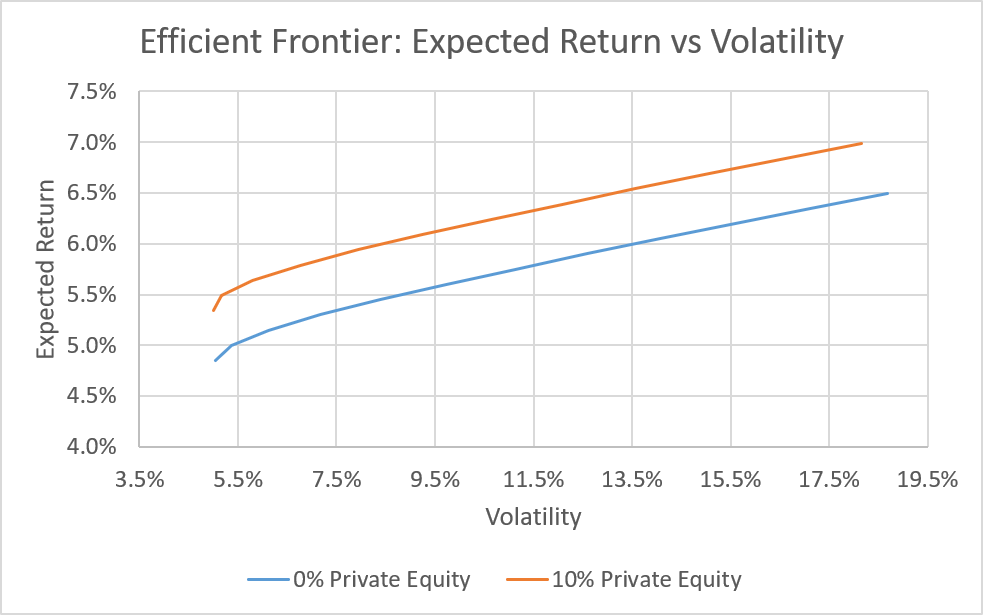
Let us reiterate the proper interpretation of this graph. The y-axis shows expected returns. These are a guess as to the mean of the return of each portfolio in the future. The actual future realized return of each portfolio can be very different from the expected return estimate, and in particular can be substantially lower than the expected return. Also in generating this graph we used capital market assumptions from KKR and MSCI (see Appendix). Nothing in the above graph represents an actual QuantStreet portfolio and the expected returns do not represent QuantStreet’s views of these asset classes. This exercise is simply to demonstrate the industry-standard argument that alternatives improve the risk-return characteristics of investor portfolios. Many asset managers have made a similar argument; see, for example, the new joint venture from Wellington, Vanguard, and Blackstone.

Before deciding to invest in alternatives, we strongly recommend that you read all (or many) of the columns Jason Zweig from the Wall Street Journal has written about this topic, starting with his recent column on why you shouldn’t blindly follow your advisor’s advice to invest in alternatives.

In addition to the excellent work of Jason Zweig, there are several other caveats which you should consider.

We used capital market assumptions from KKR to generate the above graph. Given its business model (of managing alternatives funds), KKR clearly has an incentive to show favorable return assumptions for private equity. (Though other capital market assumptions, for example, BlackRock’s, are qualitatively similar.)
Historical returns reported by all private markets managers rely heavily on their own, internal valuations for the assets they hold in their portfolio. This is known as mark-to-model, as opposed to mark-to-market (when publicly traded prices are available). Obviously, private asset managers have an incentive to overstate their valuations and understate the volatility of their returns, though there are many guardrails in place to ensure that their marks are reasonable (such as internal valuation committees, external valuation firms, and external auditors). The ultimate guardrail, of course, is the sales price at which an asset exits the portfolio.
Private equity funds are opaque. There is some visibility into the portfolios, but ultimately a lot of the investment thesis relies on trusting the portfolio manager to make good future investment decisions. There is much less transparency than what is available for typical ETFs or mutual funds.
Alternatives charge very high fees, with all-in expense ratios often in the range of 3-4% of assets under management on an annual basis. (See the Summary of Fees and Expenses in Apollo ASPM’s prospectus and Carlyle CAPM’s prospectus for a representative range for evergreen funds.) This is much higher than the fees of large, liquid ETFs offered by companies like Vanguard and BlackRock, which are often less than one tenth of one percent (e.g., BlackRock’s S&P 500 IVV ETF has a 0.03% annual expense ratio).
Alternatives are illiquid. Among the most liquid structures available to investors are tender offer evergreen funds, which offer only 3-5% quarterly liquidity at the fund level (i.e., the fund manager offers to buy back 3-5% in aggregate of the fund’s assets under management each quarter). And this liquidity provision is entirely at the discretion of the fund sponsor; the sponsor can suspend the liquidity provision if they would like, though at the expense of some reputational damage. You should never assume that you can get your money out of alternative investments as quickly as you can get your money out of public markets.
Finally, private equity funds have underperformed public markets for the last decade (see this article from the Financial Times or this one from the Wall Street Journal). Consider this table from the above July 21 2026 FT article:

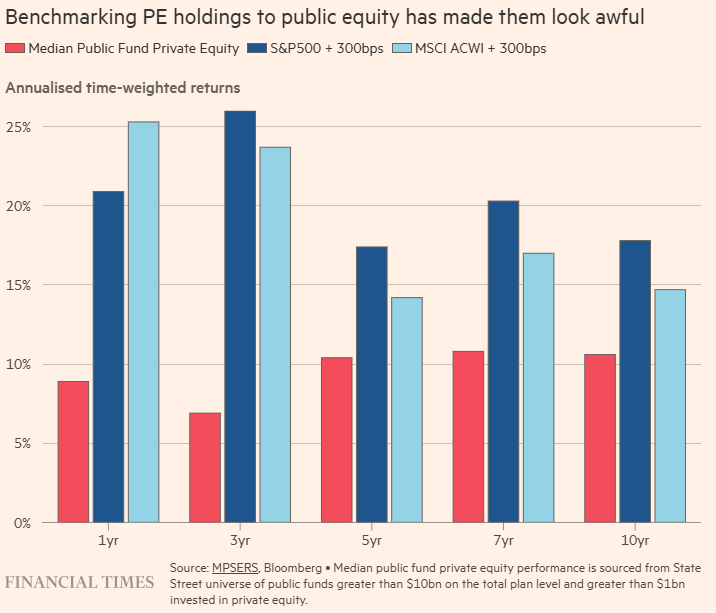
It shows that private equity has underperformed a public market + 3% benchmark over the prior 1-, 3-, 5-, 7-, and 10-year periods.

Given all of these negatives, why would anyone invest in alternatives? The pros are that, over some time periods in the past, alternatives did outperform public markets. A lot of smart investors have large allocations to alternatives (see this piece from CAIA on endowment allocations). Goldman Sachs and Bank of America both estimate that high net worth investors have, on average, 8% to 15% of their portfolios allocated to alternatives. Having a small allocation to alternatives would benefit investors if alternatives were again to outperform public markets in the future. Though should the outperformance of public markets continue, then an allocation to alternatives would be detrimental to portfolios. Keep in mind that given the complexity of alternatives and the many different ways there are of investing in them, careful due diligence is a must.

Incentive Stock Options

Following a liquidity event, employees and executives may still hold vested (and unvested) incentive stock option (ISO) awards and must decide whether to exercise or continue holding these options. There are two important considerations here. The first is to understand how valuable it is to continue to hold on to the option grant rather than exercise it. The second is to consider the tax angle of the transaction.

Let’s construct an illustrative (and purely fictional) example to investigate some of the issues. Imagine Alice owns 100,000 ISOs (vested in keeping with the $100k ISO limit as explained in the ISO Appendix), each with a ten-year maturity, a strike price of $5, with the value of the company’s stock sitting at $10 (this can be either a public market trading price or the company’s “fair market value”).

The value of an option consists of two parts. The first is the option’s intrinsic value, which is the difference between the stock price (i.e., where the stock can be sold immediately) and the option’s strike price (i.e., where the stock can be bought by the option holder). But in addition to the intrinsic value, the option also has time value. The time value arises because the option’s payoff is asymmetric. If the stock appreciates in the future, the option holder has the right to buy the stock at the same low strike price as today. But if the stock price declines in the future, the option holder’s potential loss is limited to the current value of the option, e.g., if the option ends up worthless at expiration because the stock trades below the strike price. Exercising early yields the intrinsic value to the option holder, but the time value disappears.

Should Alice exercise her options now? That depends on the time value of the option. Here, we have to make some modeling choices and then apply the well-known Black-Scholes-Merton option pricing formula to determine the option’s value. We already know the options have a 10-year lifespan, with a strike of $5 and a current stock price of $10 (or the current fair market value of $10). The other ingredients needed to price the options are an interest rate level and a volatility. Let’s use a 10-year rate of 4.7% (the current 10-year Treasury yield) and a volatility of 32.5% (roughly in line with Microsoft’s 2.5-year options and probably an understatement for a startup). We also assume the stock pays no dividend, which is reasonable in the case of most startups. In practice, you would want to check the value of the options using different levels of volatility, since we don’t know the exact volatility level at which the stock will move in the future and we assume there isn’t a traded market for these options, where the volatility can be observed.

Under these assumptions, the Black-Scholes-Merton value of each option is $7.21. Given that Alice owns 100,000 of these options, their total value is $721,000, of which $500,000 is the intrinsic value (i.e., 100,000 times the difference between the current $10 stock price/value and the $5 strike price). The options therefore have $221,000 of time value. This is the pre-tax time value of the option. Because the option exercise will lead to a complex set of taxable events (that we discuss in the ISO Appendix), the post-tax time value of the option will be lower than $221,000 but it will still be a meaningful number (in the worst case, if the option exercise and sale only generate ordinary income, this would be lower by Alice’s federal and state marginal tax rates). It is, therefore, not beneficial for Alice to exercise the option grant now and give up its large time value. (Though there is a caveat here as well, having to do with Alice’s risk aversion and liquidity needs—things that need to be assessed on a case-by-case basis.)

The tax angle of the option exercise transaction requires making several more modeling assumptions, like whether Alice is married or single, what is the household income now and in the future, and so on. One important consideration with ISOs is that exercising the option and holding the stock for over one year after exercise (and over two years after the grant date) means the sales profit above the strike price will count as a long-term capital gain, and will thus receive more favorable tax treatment. This, however, is made more complicated by the Alternative Minimum Tax. This all gets technical pretty quickly and we leave the tax analysis—and the related question of bearing another year of single-stock risk—for the ISO Appendix. (The ISO Appendix is password protected for compliance reasons. Please reach out to us if you would like to have access.)

In practice, the decision of whether to exercise a vested ISO or not should involve both your financial advisor and your accountant, working together to figure out the optimal strategy given your specific circumstances.

Conclusion

In addition to thinking about risk levels and portfolio allocations, the role of alternatives, and exercise policies for remaining incentive stock options, many additional considerations arise following a liquidity event:

Creating an estate plan and will;
Setting up trusts (especially relevant for early-stage employees or founders);
Creating tax-advantaged accounts, like 529 plans;
Supporting charitable causes;
Home purchases;
Among other considerations.

A capable team consisting of a financial advisor, an accountant, and an estate attorney should be able to help investors navigate these and other issues.

Working with QuantStreet

QuantStreet offers financial planning and wealth management services for individuals and families. For the advisor community, we offer model portfolios, portfolio analytics, and a platform for those looking to gain independence. The firm’s investment approach is systematic, data-driven, and shaped by years of investing experience. To work with or learn more about QuantStreet, join our mailing list or contact us at hello@quantstreetcapital.com. Also, please sign up for our Substack.

QuantStreet is a registered investment advisor. Registration does not imply a certain level of skill or training. All financial forecasts are fraught with risk and uncertainty. Our views may prove incorrect and market outcomes may be materially worse than we anticipate. Please see our full disclosure about the limitations of forward-looking statements and the risks of investing at https://quantstreetcapital.com/blog_disclosure/.

Appendix on Calculating the Efficient Frontier

We use expected return and volatility estimates from KKR’s capital market assumptions website (we use their 5-year ahead expected returns and their unsmoothed volatilities, which increase the anticipated volatility for private equity investments relative to the reported numbers). The correlation assumptions for US stocks, US Treasuries, and private equity are obtained from MSCI. Importantly, these are not our forecasts for future returns, but rather represent assumptions made by others in the financial industry. This analysis does not reflect any QuantStreet portfolio and is only meant to demonstrate the potential benefit of adding alternatives to traditional stock-bond portfolios. Actual future returns and volatilities of these asset classes may be worse (i.e., lower returns and higher volatilities) than the assumptions used in the above analysis.